The Elman RNN

Introduction

This relates the experience of implementing an Elman network for modeling sequential information.

The Elman network was introduced by Jeffrey L. Elman in a 1990 paper titled Finding Structure in Time. It uses ideas very similar to those introduced by Michael I. Jordan in a 1986 technical report.

The Jordan and Elman models address a basic limitation of multilayer perceptrons: the input size and number of layers (processing steps) is fixed. This can be a problem when processing sequential inputs where the input size is variable (e.g. speech, sound, time series …). Jordan’s idea was to go go through the inputs one at a time, and having a state layer that maintains information about the previous inputs up to this point. To implement this state, the inputs to the network are expanded with a state layer whose inputs are the outputs of the network at the previous time step. In other words, the inputs to the hidden layer at time $t$ include the outputs of the network at time $t-1$.

The Elman network, also known as the SRN or Simple Recurrent Network is very similar. The difference is that the input to the hidden layer, instead of receiving a copy of the network’s output, receives a copy of the hidden layer’s activity at the previous time step.

The task for this implementation was to learn to recreate a set of hand-drawn traces: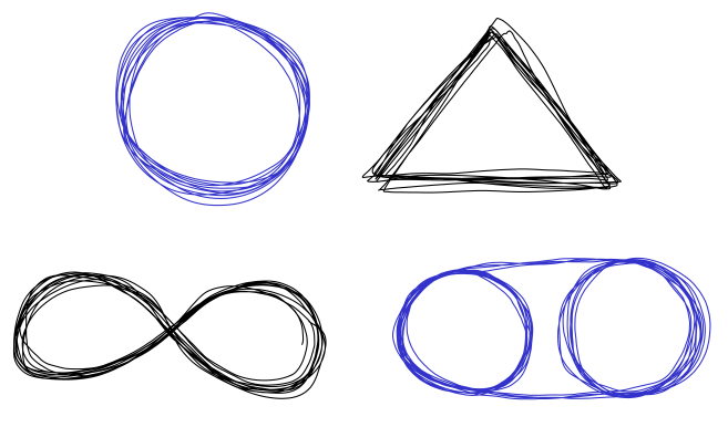

These traces were drawn by hand and exported into the .svg format. I wrote a function to extract a sequence of $(x,y)$ coordinates from the svg file, which were stored in Numpy array with roughly 1000 rows and 2 columns. The task of the network was to learn this sequence of traces, but due to the noisy nature of hand drawing the network must create limit cycle attractors that roughly follow the mean trajectory of the lines.

The circle and the triangle are the simplest examples for one reason: to predict the coordinates at the next time point all you require are the $(x, y)$ coordinates at the current time. This is especially true when $(x, y)$ is close to the “mean trajectory”. In theory a multilayer perceptron could learn to trace these shapes.

The figure eight (infinity symbol) self intersects, and at the intersection point you need some memory of the previous points in order to predict what is the next coordinate in the trajectory. This pattern thus requires some memory, and the Elman network seems just right for the task.

The figure on the bottom right is the most challenging one. The trace begins by doing circle on the left. After 2.5 circular revolutions the trace moves to the right and begins another circle. Every 2.5 revolutions the circle is switched. Learning to predict the next point requires a much longer memory now, enough to remember how many circular revolutions have been completed on the current side. Such a memory requirement strains the memory capacity of the Elman network, and motivates the introduction of the Multiple-Timescales RNN, described in a subsequent blog post.

Results

I implemented a basic Elman RNN using Python and Pytorch. Source code is here. For the purpose of this exploration I used a hidden layer with 50 units, tanh nonlinearity, the Adam optimizer, and a learning rate of 3e-4.

First, let’s look at the circle.

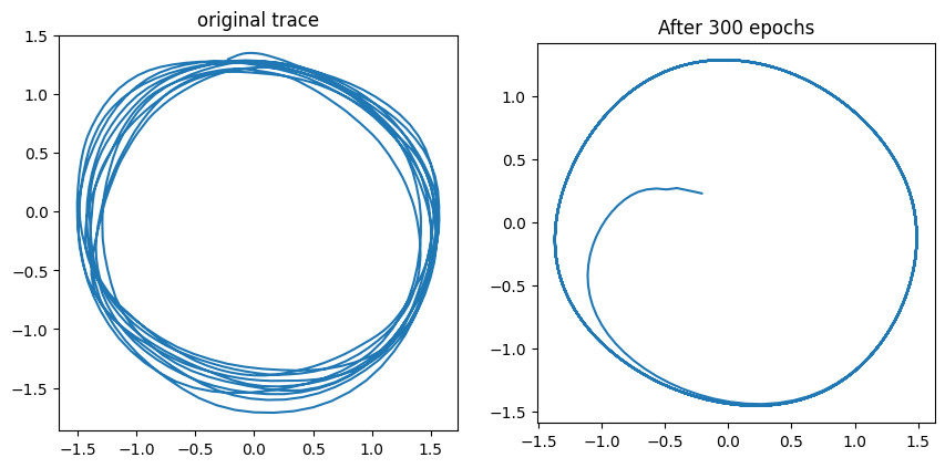
To generate the panel on the right the trained Elman network was given an initial coordinate ($x=0, y=0$), and an initial state for the hidden layer (all activity set to zero). The trace on the panel was created by recursively feeding the output at time step $t$ as the input for time step $t+1$. We can see that after 300 epochs of training we have a nice limit cycle attractor as emerged.

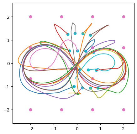
A few more initial conditions can be seen in this figure:

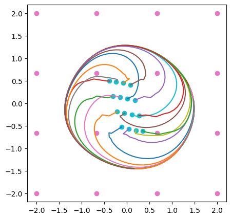
The pink dots in the figure represent the initial coordinates given to the Elman network; in this case a 4 x 4 grid of values. The cyan dots show the first point produced for all the 16 initial conditions. The large discontinuous jump from the pink to the cyan dots is a reminder that the recurrent trace generation done here is a discrete process, not a continuous one. Moreover, this plot should not be interepreted as a phase diagram. As a dynamical system, the recurrent process is 52-dimensional, so its flow can’t entirely be captured in 2 dimensions. All the trajectories shown here start from the point where the hidden units have zero activity.

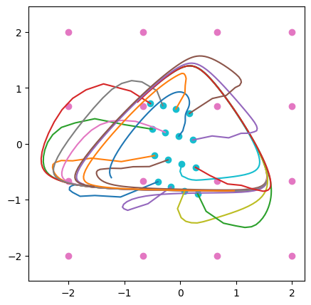
With those caveats being said, it is clear from the figure that a large number of initial conditions are attracted to the circular trajectory. The case of learning to trace a triangle is very similar, as can be observed in the figures below.

The infinity symbol took many more epochs to learn:

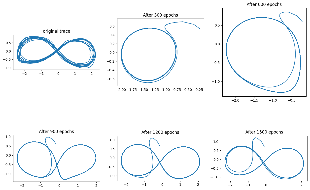
Initially the network settled into a roughly circular attractor, and it took many cycles of training before this trajectory could be deformed into a self-intersecting shape.

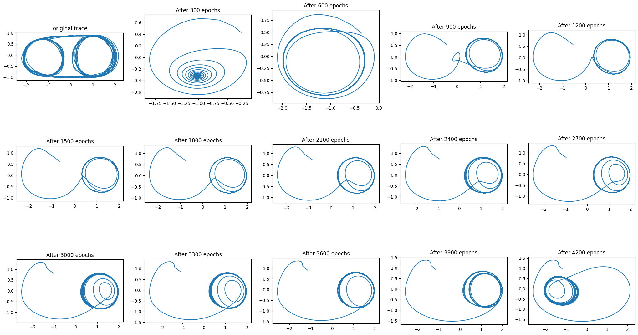
Finally, I attempted to learn to predict the trajectory where the circular motions switch sides every 2.5 cycles. As can be seen below, the network tried to approximate the shape, and even seems to have learned separate attractors for the circles on the right and the left, but trajectories settled on a single circle and didn’t switch sides.

Bonus round: LSTM

The problem here is that we need information about the trajectory’s history far in the past. This is precisely the type of problem that LSTMs are meant to solve. As a bonus, I quickly replaced the Elman RNN for an LSTM network. There was no parameter tuning whatsoever, so consider that when seeing the next figure:

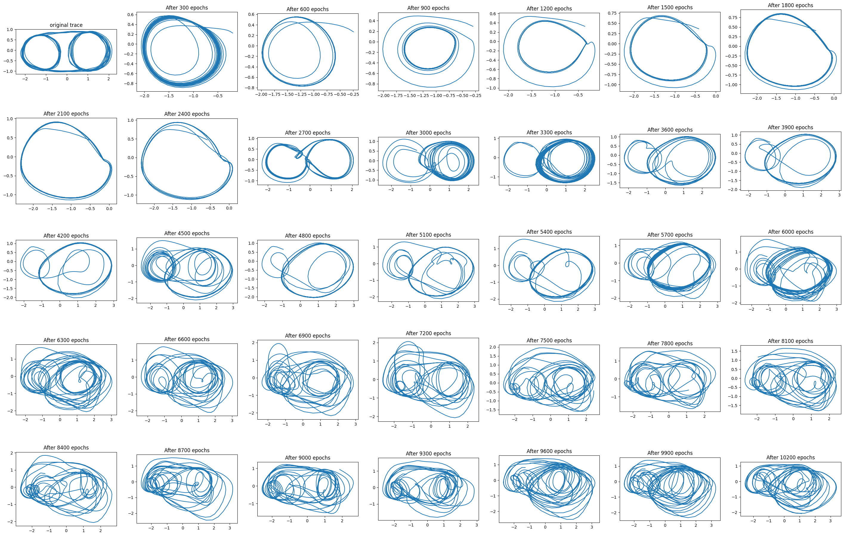
My impression is that LSTM can indeed solve this problem, although the current parameters aren’t particularly effective. I was able to run 10200 epochs because the Pytorch LSTM implementation is seriously fast.