Multiple-Timescales Recurrent Neural Networks (MTRNNs)

Introduction

This post is a continuation of my previous post on Elman networks.

The MTRNN is a network architecture capable of learning long time dependencies more effectively than an Elman network. This architecture is described in Yamashita and Tani 2010, Emergence of Functional Hierarchy in a Multiple Timescale Neural Network Model: A Humanoid Robot Experiment.

This is very similar to a cascade of Elman or Jordan recurrent networks, with the key difference that the networks are now considered to operate in continuous time, and the units in the higher levels have slower (larger) time constants.

I made a simple adaptation of the network in Yamshita and Tani 2010 for the problem of learning traces (sequences of 2D coordinates). The basic architecture is in the next figure.

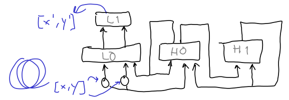
As in the Elman RNN post, the input to the network is a sequence of $(x, y)$ coordinates, and the output is a prediction of the coordinates $(x’, y’)$ at the next time step. L0 is a fully-connected layer, using $tanh$ nonlinearities in this implementation. L1 is a linear layer. H0 and H1 are Elman RNN cells with fast and slow timescales, respectively.

A difference with the Yamashita and Tani 2010 network is that in here outputs come from a linear layer, rather than a softmax layer. Moreover, H0 and H1 each consist of a single layer, and they update after applying the $tanh$ nonlinearity. In other words, if $\mathbf{h}_i$ denotes the activation vector of the units in hidden layer $i$, the update steps are described by:

\[\mathbf{h}_i^* = \tanh \left( \mathbf{W_i I_i} \right)\] \[\mathbf{h}_i \leftarrow \left( 1 - \frac{1}{\tau_i} \right) \mathbf{h}_i + \frac{1}{\tau_i} \mathbf{h}_i^*\]

Where $\mathbf{W}_i$ and $\mathbf{I}_i$ are respectively the weight matrix and input vector for hidden layer $i$. As a curious note, initially I made a mistake when wrting the equations to update the activity, so the update was: $\mathbf{h}_i \leftarrow \left( 1 - \frac{1}{\tau_i} \right) \mathbf{h}_i^*$. The network with this update rule could still learn to approximate circles, triangles, and with some work even figure eights. This is probably because the network with these update equations is like two stacked Elman networks with some error in the activation. It serves to illustrate a valuable lesson, so I threw this result in an Appendix at the bottom of this post.

Going back to the network with the correct equations, I used layer sizes of 10, 40, 8 for L0, H0, and H1, respectively. The time constant for H0 was 4, and the one for H1 was 80. The optimizer was Adam with time constant 3e-4.

Results

Like the Elman network, the MTRNN could learn to trace circles, triangles, and infinity symbols. This is very similar to the case with the Elman network, so I’ll only show a single result.

In this case it can be seen that the self-intersection does not prevent learning. The attractors produced by the Elman network seemed “cleaner”, however. It is possible that the MTRNN, with its higher memory capacity, was learning to reproduce some of the quirks in the hand-drawn image (overfitting).

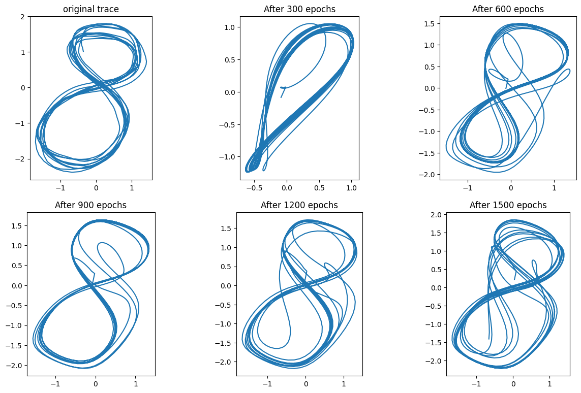
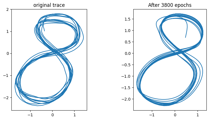
Training for a longer period suggests that this may be the case. The attractors produced by the Elman network seemed to be limit cycles whose period coincided with the periodicity of the trajectory in the drawing. In the case of the MTRNN, the attractor seems to be a limit cycle that spans several loops (the original trace contains 10 loops).

The more interesting part is the trace where the side switches every few revolutions, requiring a longer memory of the trajectory. The result for this case can be seen below.

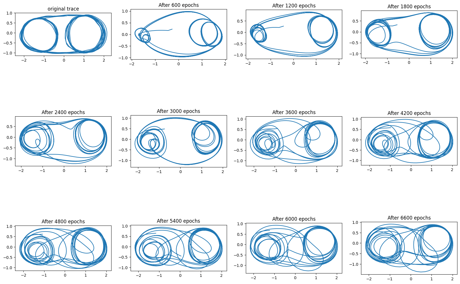
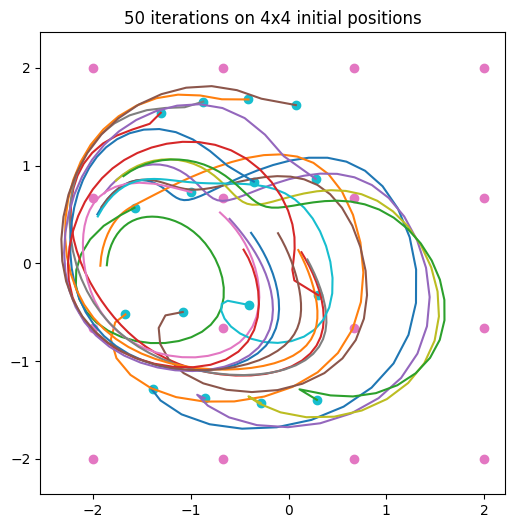
After 6600 epochs the trajectory switched sides while still making a loop, which made the plot messy. But clearly this was not separate attractors on each side, as in the case of the Elman network. There was a single attractor that for initial states with zeros in the hidden layers started its trajectory by looping on the left side, and then shifted to the right. Partial trajectories for a few initial states can be seen in the figure below.

Some thoughts

I did very little in terms of optimizing these hyperparameters but I still came out wondering whether there is a principled way to obtain good values for the various time constants. Perhaps along the lines of extracting the Fourier coefficients of the incoming inputs. Large coefficients for slow frequencies would cause time constants to increase, etc.

Appendix: Incorrect equations, but so-so results

Before I realized that my MTRNN had the wrong equations I tried to teach it a pattern consisting of 5 circular revolutions on the left, followed by 5 revolutions on the right, then back to the left, and so on.

The network was reducing the error during training, but it became clear that when generating trajectories it didn’t learn to complete 5 revolutions on one side, and then go to the other side. This prompted me to increase the number of epochs. After 10000 epochs the error reached a very small value (~8e-05), and the results can be seen below:

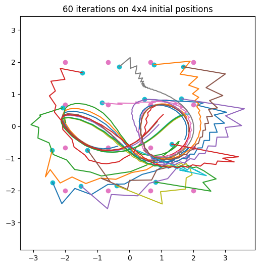
It can be observed that the network learned to trace multiple revolutions on the left, before finally settling on the limit-cycle attractor on the right, from which it can’t escape. This is still not the desired pattern, but an interesting approximation nonetheless.

One thing this example shows is that the ability of backpropagation to reduce the loss can mask errors in the code. In the words of Andrej Karpathy:

It is a depressing fact that your network will typically still train okay…

That’s one reason he recommends an evaluation skeleton and many sanity checks in his Recipe for Training Neural Networks.