The variational autoencoder from scratch: an exercise in balance

In this post I wrote some thoughts on what the Variational Autoencoder (VAE) is supposed to do, and on ideas I got while programming it from scratch.

A lot of these thoughts were motivated by reading Doersch 2017, which was my entry point to VAEs.

Source code for my VAE implementation (which is not particularly clean) is located here. Source code from people who know what they’re doing can be seen here.

Preamble

A lot of the work in statistical machine learning is focused on learning a distribution $p(\mathbf{x})$ based on a collection of examples ${ \mathbf{x}_1, \dots, \mathbf{x}_n }$. These examples could be things like faces or sentences, and an interesting thing about having $p(\mathbf{x})$ is that then you can sample from that distribution, to generate synthetic faces or sentences.

Some people get excited about learning a distribution and sampling from it. Perhaps because in some sense this captures the process that generates the samples, so the distribution models an aspect of the world and its uncertainty. The problem is that the sample space is just too big in the interesting cases. How many 512x512 RGB images are possible?

An approach to make distributions tractable is to extract latent variables. Ideally, these variables are related to the process that generates the $\mathbf{x}$ data points, and can encode their distribution with dramatically reduced dimensionality. For example, if the data points are images of digits, a single variable with the identity of the digit (0-9) would go a long way in capturing the relevant information in the image.

Working with latent variables (denoted here by $\mathbf{z}$) has at least two big challenges. The first is deciding what the variable will encode. Which features can capture the information in the training data? The second challenge is to obtain the distribution $p(\mathbf{z})$. Obtaining this distribution is important because once you know it you can take samples of $\mathbf{z}$, and with with the help of a decoder (mapping values of $\mathbf{z}$ to their corresponding value of $\mathbf{x}$) you can generate synthetic data, as if you were sampling from $p(\mathbf{x})$.

The VAE

The variational autoencoder is an architecture capable of learning the latent variables $\mathbf{z}$ that correspond to a given input $\mathbf{x}$ (in other words, approximately learning the distribution \(p(\mathbf{z} \vert \mathbf{x})\)), and of producing a decoder network that, given $\mathbf{z}$, yields a corresponding value of $\mathbf{x}$. Moreover, the $\mathbf{z}$ variables it learns are such that $p(\mathbf{z})$ is close to a multivariate normal distribution, so we can sample $\mathbf{z}$ values and feed them to the decoder in order to produce synthetic data!

I’ll skip all the math (there are better explanations out there), and jump into what the VAE is computationally, what is the intuition, and how you train it.

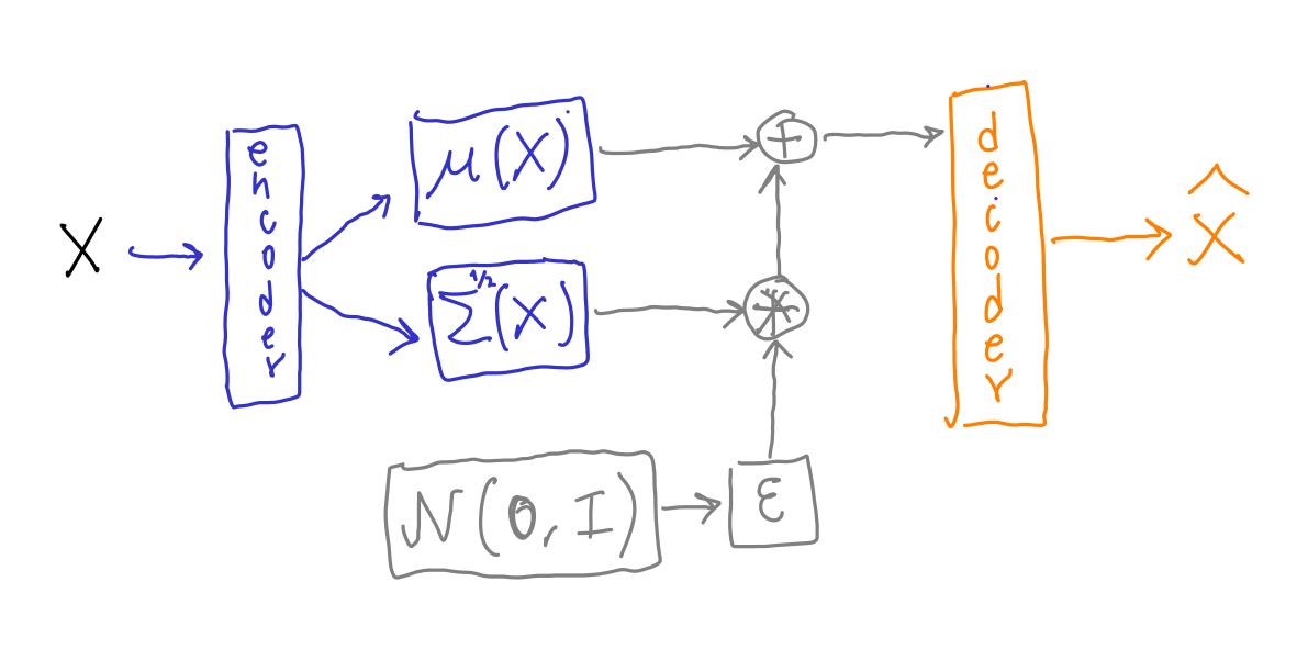
The VAE is this stochastic machine:

This machine takes the original high-dimensional input $\mathbf{x}$ (e.g. images), and stochastically produces a “reconstructed” version of $\mathbf{x}$, denoted by $\hat{\mathbf{x}}$.

The encoder is some neural network that receives $\mathbf{x}$ and outputs two vectors $\mu(\mathbf{x}), \text{diag}\left(\Sigma^{1/2}(\mathbf{x})\right)$. Each of these two vectors has $n_z$ elements, with $n_z$ being the number of latent variables. $\mu(\mathbf{x})$ and $\text{diag}\left(\Sigma^{1/2}(\mathbf{x})\right)$ are the parameters of a multivariate normal distribution that will be used to stochastically generate $\mathbf{z}$ by sampling from it. This normal distribution is assumed to have a diagonal covariance matrix $\Sigma$, so we only need $n_z$ elements to represent it using the vector $\text{diag}\left(\Sigma^{1/2}\right)$. The vector $\mu$ contains the means of the distribution.

Sampling from the multivariate normal during training is done in a sneaky way. Rather than sampling directly from $\mathcal{N}(\mu, \Sigma)$ we sample a vector $\mathbf{\varepsilon}$ from a standard multivariate normal distribution $\mathcal{N}(\mathbf{0}, \mathbf{I})$ (zero mean and identity covariance matrix). Then the sample is produced as \(\mathbf{z} = \mu(\mathbf{x}) + \mathbf{\varepsilon} * \Sigma^{1/2}(\mathbf{x})\) What this achieves is to make the path of computations from $\mathbf{x}$ to $\hat{\mathbf{x}}$ entirely differentiable, which allows us to do backpropagation using the $|\mathbf{x} - \hat{\mathbf{x}}|^2$ reconstruction error. Error measures different from mean-squared error may be used, but the idea is the same. Had we sampled directly from $\mathcal{N}(\mu(\mathbf{x}), \Sigma^{1/2}(\mathbf{x}))$ the non-differentiable random sampling part would have blocked backpropagation of gradients. This sneaky sampling is known as the reparameterization trick.

The decoder is a neural network that takes $\mathbf{z}$ and outputs $\hat{\mathbf{x}}$.

At this point we are in position to train both the decoder and the encoder using backpropagation and the reconstruction error. But if we only use this error then the VAE will still not allow us to generate synthetic outputs by sampling $\mathbf{z}$. Why? Because the distribution of $\mathbf{z}$ that we use for training is different (has different $\mu, \Sigma$ parameters) for every value of $\mathbf{x}$. Which distribution can use use for sampling $\mathbf{z}$ to generate data?

The solution is to train the encoder so that $\mathbf{z}$ has a known, simple distribution $p(\mathbf{z})$ that allows sampling. In the most common version of the VAE we assume that the true distribution $p(\mathbf{z})$ is $\mathcal{N}(\mathbf{0}, \mathbf{I})$. Since $p(\mathbf{x})$ will usually not be anything like a standard normal, it is really unlikely that the output $\mu, \Sigma$ of the encoder will be anything like a standard normal distribution when the encoder’s parameters are being adjusted only to reduce the reconstruction error.

In reality the encoder will produce an output with distribution $q(\mathbf{z})$. We would like to modify the weights of the decoder so not only is the reconstruction error is minimized, but also $q(\mathbf{z})$ gets close to a standard normal distribution. Thus, the loss function for the encoder needs another term that quantifies the difference between $q(\mathbf{z})$ and $\mathcal{N}(\mathbf{0}, \mathbf{I})$. When you want to quantify the difference between two distributions the usual measure is the Kullback-Leibler divergence, and this is what the VAE uses.

Thus you’ll have a term $\text{KL}[q(\mathbf{z}) | p(\mathbf{z})]$ in the decoder’s loss, but estimating $q(\mathbf{z})$ is still computationally expensive, so what you’ll do is to use $\text{KL}[q(\mathbf{z} \vert \mathbf{x}) | p(\mathbf{z})]$ repeatedly. In other words, for each point $\mathbf{x}$ in the training data you’ll produce gradients so the encoder produces values $\mu(\mathbf{x}), \Sigma^{1/2}(\mathbf{x})$ closer to $\mathbf{0}, \mathbf{1}$. This tendency to produce values of $\mu, \Sigma$ that are just vectors with zeros and ones must be balanced with the requirement of $\mu(\mathbf{x}), \Sigma(\mathbf{x})$ still maintaining information about $\mathbf{x}$, so the decoder can reconstruct it.

Results

I wrote a version of the VAE based on equation 7 in Doersch 2017. In particular: \(\text{KL}(q(\mathbf{z \vert \mathbf{x}}) \| \mathcal{N}(\mathbf{0}, I)) = \frac{1}{2}\left(\text{tr}(\Sigma(\mathbf{x}) + \mu(\mathbf{x})^T \mu(\mathbf{x}) -k - \text{log det}(\Sigma(\mathbf{x}))) \right)\)

The loss function was the sum of the reconstruction error plus this divergence \(\mathcal{L} = \|\mathbf{x} - \mathbf{\hat{x}} \|^2 + \text{KL}(q(\mathbf{z|\mathbf{x}}) \| \mathcal{N}(\mathbf{0}, I)) \equiv RE + DE\)

where RE stands for “Reconstruction Error”, and DE stands for “Distribution Error”. Notice that $q$ does not depend on the parameters of the decoder. The derivative of the DE only affects the parameters of the encoder, whereas the derivative of RE affects both encoder and decoder.

I trained the encoder to produce $\mu, \text{diag}(\Sigma)$ values. Unbeknownst to me, most implementations of the VAE follow the original Kingma and Welling 2013 derivation, in which the encoder outputs the logarithm of $\mu$ and $\Sigma$. This shouldn’t affect the direction of backpropagation, but in practice it has the effect that it changes the relative magnitude of the two errors in the loss function.

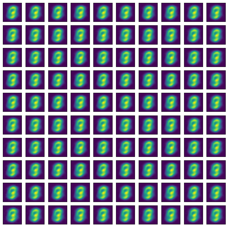
The first time that I trained my VAE to produce images of digits based on the MNIST dataset all the samples would produce the same image, which looked a bit like an “average number”.

The VAE for this image has a 2D latent variable $\mathbf{z}$, and there is a 10x10 grid of $\mathbf{z}$ values where each dimension ranges from -2 to 2. Training proceeded for 10 epochs.

How to fix this?

A first clue was that the reconstruction error was more than one order of magnitude smaller than the distribution error. My guess is that reducing the reconstruction error too aggressively caused training to enter an attractor from which it couldn’t escape, because the escape routes involved increasing RE for a few iterations.

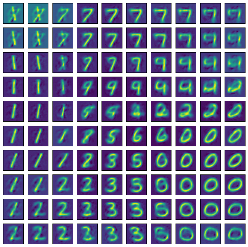
The easy fix was to modify the loss function as \(\mathcal{L} = RE + w \cdot DE\) where $w=0.001$. This allowed reconstruction of the digits.

Finding a good value of $w$ was quite time consuming. I decided to try to automate this process using this criterion: on average, $RE$ should have a similar magnitude to $w RE$. In other words, at every iteration slightly modify $w$ so that $\frac{wDE}{RE} \approx 1$. The ratio of 1 is an arbitrary quantity, but worked well for this example.

What I did was to start with $w=0$, and then on every minibatch to adust its value as \(\Delta w = \alpha (RE - wDE)\) with $\alpha = 10^{-5}$.

I did’t know it at the time, but what I had conjured was a variation of the KL cost annealing introduced in this paper (Bowman et al. 2015, “Generating sentences from a continuous space”).

Bonus:

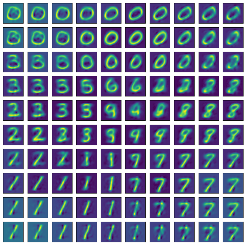
Using a single latent variable we get

A lot of information gets stored in a single $z$ value!