Variational Recurrent Neural Network (VRNN): not your regular RNN

In this post I try to explain the ideas behind the Variational Recurrent Neural Network, and convey the experiences from implementing one with PyTorch.

Rather than getting to the point, I relate the beginner errors I introduced into my program, which frustrated me for days. Also I write some of the rambling ideas I had during the process.

Introduction

In two previous posts I played with RNNs for modeling sequential data. In particular, these networks could learn attractors that required significant memory of previous states.

The RNNs I used, when recursively generating sequential data (when the output from time $t-1$ became the input at time $t$), constituted deterministic discrete dynamical systems. They do not have the ability to model a process that is inherently stochastic.

For example, suppose we are generating 2D trajectories with the following procedure: we trace 2 revolutions of a circle (pattern A), and then we trace a triangle twice (pattern B). At this point with 33% chance we repeat pattern B, with 33% chance we do a figure eight twice (pattern C), or with 33% chance we return to pattern A. After pattern C we always return to pattern A.

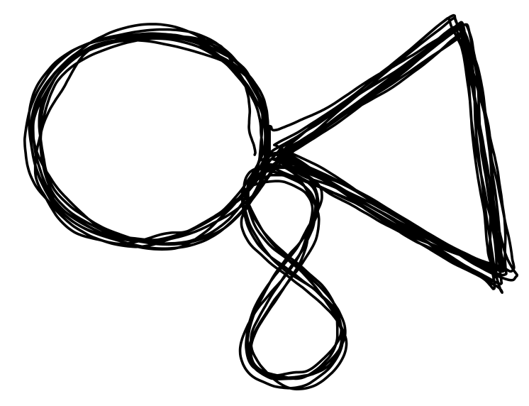
The figure above goes through patterns A, B, A, B, C, A, B, B, C, A (or something like that). This is like a non-deterministic finite automaton where the transitions from A to B and from C to A are deterministic, but the transitions from B are stochastic, and can go to any other state with equal probability.

If what you want is to generate non-repeating valid sequences containing the A, B, C patterns, a deterministic RNN has no way of learning the probabily of a transition.

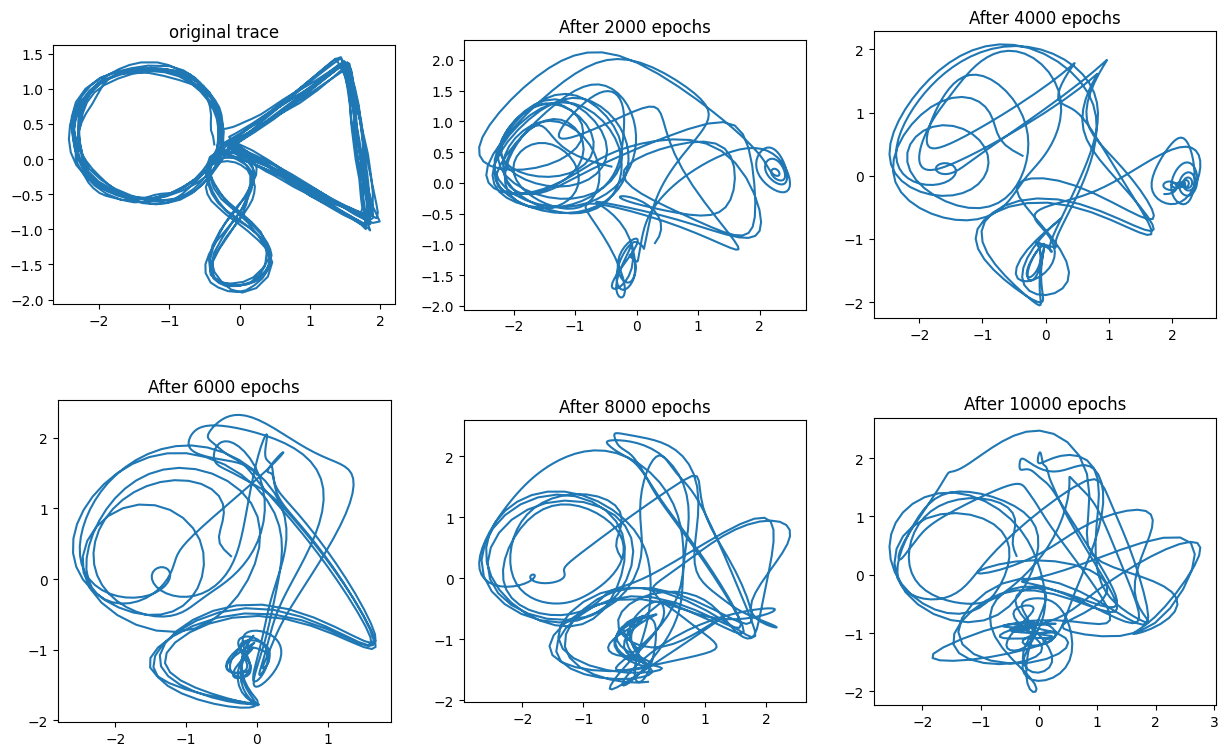
Here is how the MTRNN fares when trying to learn the pattern of the figure above. Because the pattern is not periodic, it must learn to reproduce the whole trace in order to make a similar figure.

On the other hand, the variational autoencoder (VAE) is capable of learning complex distributions and producing samples from them, but the standard VAE is not appropriate for modeling sequential data. Just like feedforward perceptrons, the VAE has a fixed input and output size, so taking inputs of varying lengths, or generating very long output sequences is problematic.

If we could only combine the distribution-learning ability of the VAE with the RNNs’ ability to handle sequences…

The Variational Recurrent Neural Network (VRNN)

Your typical RNN works through repeated applications of a cell, that at time $t$ takes an input $x_t$ and the previous hidden state $h_{t-1}$. With this the cell produces a hidden state $h_{t}$ and an output $y_t$. Usually the cell is an LSTM or GRU layer. But what if our cell was a VAE?

This is the premise of the VRNN, introduced in 2015 by Chung et al. The way it works is a combination of the procedures for using RNNs and VAEs. There are only 3 extra elements:

• There is is an intermediate extraction of features for the input $\mathbf{x}_t$ and the latent variable $\mathbf{z}_t$, which the authors claim is required for good performance.
• The normal distribution generating \(\mathbf{z}_t\) is no longer assumed to always have mean $\mathbf{0}$ and identity covariance matrix. Instead, the mean and the (diagonal) covariance matrix will depend on the previous hidden state $\mathbf{h}_{t-1}$. According to the authors, this secret sauce gives the model better representational power. The results support this claim, but the advantage it confers doesn’t seem to be dramatic.
• When generating samples the decoder outputs parameters of a distribution that generates $\mathbf{x}$, rather than providing $\mathbf{x}$ directly. This is not unusual in RNNs, but it’s not how the original VAE operated.

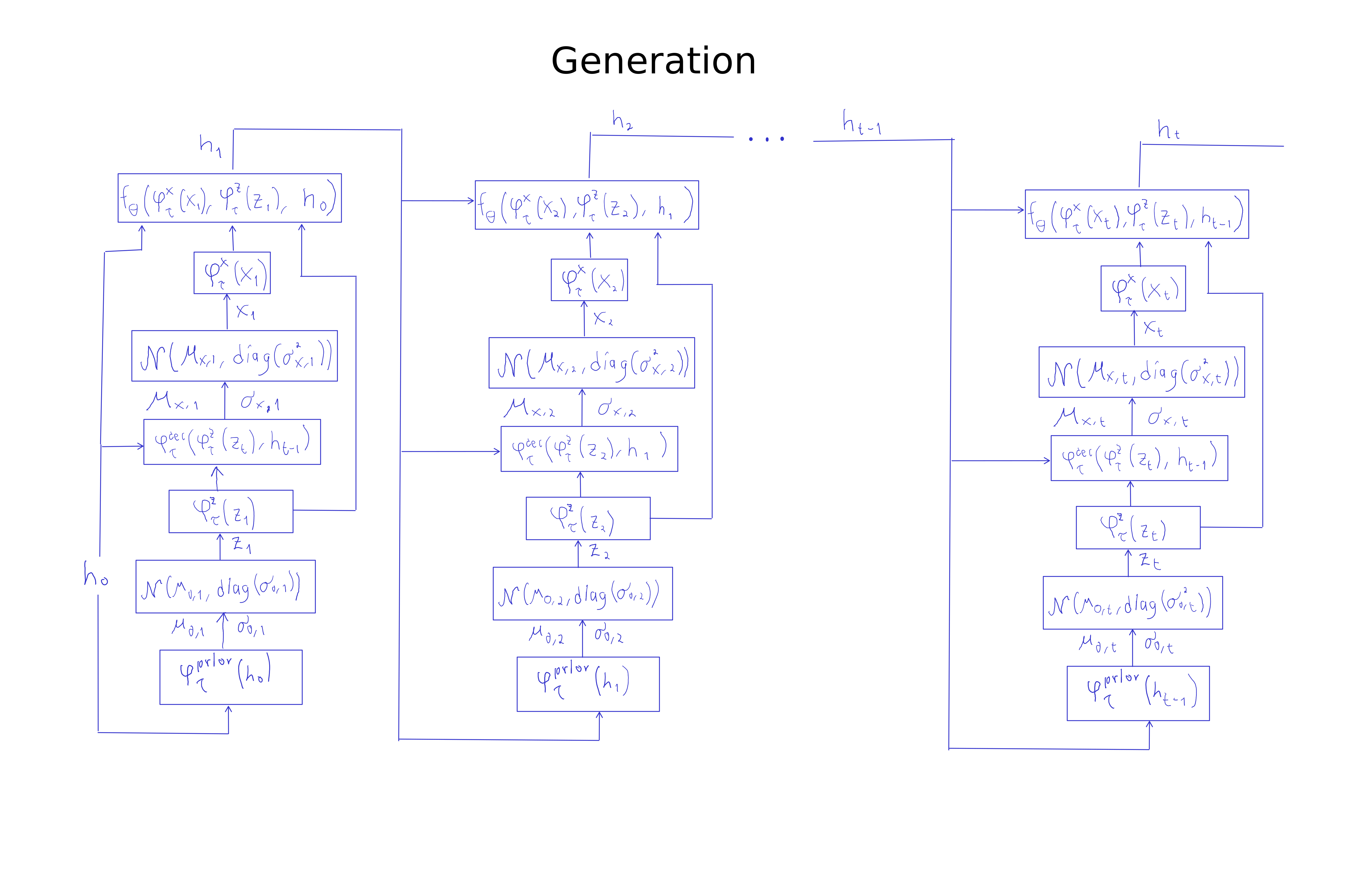
If you want to generate samples using a VRNN, you begin with an initial hidden state $\mathbf{h}_0$, usually a vector with zeros. Then:

1. Generate the first latent variable \(\mathbf{z}_1\) in two steps.
   1. Obtain the mean \(\mathbf{\mu}_{0,1}\) and covariance matrix \(\text{diag}(\mathbf{\sigma}_{0,1})\) of the prior distribution for \(\mathbf{z}\). This comes from the output of a network whose input is \(\mathbf{h}_0\), and is denoted by \(\varphi_\tau^{prior}(\mathbf{h}_0)\).
   2. Sample \(\mathbf{z}_1\) from the distribution \(\mathcal{N}(\mathbf{\mu}_{0,1},\text{diag}(\mathbf{\sigma}_{0,1}))\) (with the reparameterization trick).
2. Extract features from \(\mathbf{z}_1\) using a network denoted by \(\varphi_\tau^{z}(\mathbf{z}_1)\).
3. Obtain the first synthetic value $\mathbf{x}_1$ in two steps.
   1. Feed \(\varphi_\tau^{z}(\mathbf{z}_1)\) and $\mathbf{h}_0$ into the decoder to produce parameters \(\mathbf{\mu}_{x,1}\), \(\mathbf{\sigma}_{x,1}\).
   2. Produce a value \(\mathbf{x}_1\) by sampling from the distribution \(\mathcal{N}(\mathbf{\mu}_{x,1}, \text{diag}(\mathbf{\sigma}_{x,1}))\).
4. Extract features $\varphi_\tau^x(\mathbf{x}_1)$ using a neural network.
5. Update the hidden state: \(\mathbf{h}_1 = f_\theta\Big(\varphi_\tau^x(\mathbf{x}_1), \varphi_\tau^z(\mathbf{z}_1), \mathbf{h}_0 \Big)\)

The rest of the procedure is just a repetition of the previous steps starting with the updated hidden state. The next figure illustrates this.

The procedure for training is not very different, but now at each step $t$ you will have an input $\mathbf{x}_t$ that you will stochastically reconstruct in two broad steps by

1. Obtaining a \(\mathbf{z}_t\) value using an encoder. This approximates sampling from \(p(\mathbf{z}_t \vert \mathbf{x}_{\leq t})\).
2. Obtaining a $\hat{\mathbf{x}}_t$ value using a decoder. This approximates sampling from \(p(\mathbf{x}_t \vert \mathbf{z}_t)\).

After a full sequence \(\hat{\mathbf{x}}_1, \dots, \hat{\mathbf{x}}_{T}\) has been generated, gradient descent uses an objective function that is like the sum of $T$ VAE objective functions, one for each time step: \(\mathbb{E}_{q(\mathbf{z}_{\leq T}|\mathbf{x}_{\leq T})} \left[ \sum_{t=1}^T \Big(-\text{KL}(q(\mathbf{z}_t | \mathbf{x}_{\leq t}, \mathbf{z}_{< t}) \|p(\mathbf{z}_t | \mathbf{x}_{< t}, \mathbf{z}_{< t})) + \log p(\mathbf{x}_t | \mathbf{x}_{\leq t}, \mathbf{z}_{< t}) \Big) \right]\)

The actual flow of computations can be seen in this figure:

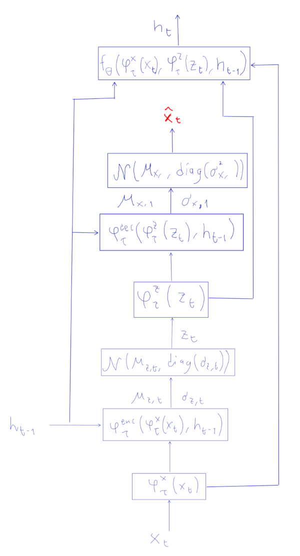
As with the VAE, we don’t actually calculate the expected values of the objective function. Instead we use stochastic gradient descent with individual sequences. A reconstruction error is used to reduce \(\log p(\mathbf{x}_t \vert \mathbf{x}_{\leq t}, \mathbf{z}_{< t})\). Not shown in the figure above is that the reparameterization trick from VAEs is used in all sampling steps.

Something that not clear from the “training computations” figure above is how we are going to train the network $\varphi_\tau^{prior}(\mathbf{h})$ that produces parameters for the prior distribution of $\mathbf{z}$ based on the previous hidden state $\mathbf{h}$. The answer is that during the forward passes in training we will also generate values \(\mathbf{\mu}_{0,t}, \mathbf{\sigma}_{0,t}\). The part of the loss function corresponding to the terms \(-\text{KL}(q(\mathbf{z}_t \vert \mathbf{x}_{\leq t}, \mathbf{z}_{< t}) \|p(\mathbf{z}_t \vert \mathbf{x}_{< t}, \mathbf{z}_{< t}))\) uses \(\mathbf{\mu}_{0,t}, \mathbf{\sigma}_{0,t}\) to characterize the distirbution of \(p(\mathbf{z}_t \vert \mathbf{x}_{< t}, \mathbf{z}_{< t})\), and \(\mathbf{\mu}_{z,t}, \mathbf{\sigma}_{z,t}\) for the variational distribution \(q(\mathbf{z}_t \vert \mathbf{x}_{\leq t}, \mathbf{z}_{< t})\).

To implement the objective KL divergence part of the objective function you just need to find what this is in the case of two multivariate Gaussians. Because I didn’t want to spend time deriving this divergence I just looked it up, and found it at the last page of this pdf (among other places).

Results

There are quite a few elements in a VRNN, so it helps to look at previous implementations. The code from the original paper uses the cle framework, which is a bit dated. Instead, I found inspiration from this PyTorch implementation. My own implementation can be seen here.

Setting metaparameters

Basically, a VRNN will use 6 networks:

1. $\varphi_\tau^x(\mathbf{x}_t)$,
2. $\varphi_\tau^{prior}(\mathbf{h}_{t-1})$,
3. \(\varphi_\tau^{enc}(\varphi_\tau^x(\mathbf{x}_t), \mathbf{h}_{t-1})\),
4. $\varphi_\tau^z(\mathbf{x}_t)$,
5. \(\varphi_\tau^{dec}(\varphi_\tau^z(\mathbf{z}_t), \mathbf{h}_{t-1})\),
6. \(f_\theta \left( \varphi_\tau^x(\mathbf{x}_t), \varphi_\tau^z(\mathbf{z}_t), \mathbf{h}_{t-1} \right)\).

To implement the VRNN you need to choose the metaparameters of these networks, and create code that applies them in the right order for inference and generation. With so many networks, choosing metaparameters is in fact one of the challenges.

Given the task of generating the “circle-triangle-eight” pattern shown above I chose parameters with this reasoning:

• $\mathbf{h}$ has to encode the basic shape of the patterns and the the current point in the cycle. 60 units should suffice.
• The latent space needs to encode the current shape, and the amount of randomness that should be involved when choosing the next point. For this I deemed that at least two variables should be used, and to be sure I set the dimension of $\mathbf{z}$ to 10.
• $\varphi^x_\tau$ and $\varphi^z_\tau$ “extract features” from $\mathbf{x}$ and $\mathbf{z}$. It seemed fitting that the number of features should be larger than the dimensions of $\mathbf{x}$ and $\mathbf{z}$, so those features could make an “explicit” representation. I set these as 1-layer networks with 10 units for \(\varphi^x_\tau\) and 16 units for \(\varphi^z_\tau\).
• $\varphi^{prior}_\tau$ must produce the distribution for the latent variables given $\mathbf{h}$. I used a network with a 30-unit hidden layer.
• \(\varphi^{enc}_\tau\) and $\varphi^{dec}_\tau$ must produce distribution parameters based on the current hidden state and on extracted features. \(\varphi^{enc}_\tau\) is a network with a 30-unit hidden layer, whereas \(\varphi^{dec}_\tau\) uses 40 units.
• In the case of $f_{\theta}$ I used a single 60-unit layer that could optionally use GRU units.

These are probably more units than necessary for the “circle-triangle-eight”, but in an initial exploration I am less concerned with overfitting, and more concerned with finding whether the network can do the task. I used smaller networks and an Elman RNN for the other experiments described below.

As with the VAE, I used Mean Squared Error loss for the reconstruction error, and set an adaptive $w$ parameter to balance the magnitude of this error with the much larger output of the KL divergence between the prior and posterior $\mathbf{z}$ distributions.

A rough start

After the code was completed the traces my network produced were random blotches. I assumed there was an error in my code, but going through each line didn’t reveal anything. After an embarrassingly long time I realized that the output of my encoder, decoder, and prior networks corresponding to means should not use ReLU units in the output layer, because then those outputs could not be negative…

Once I modified the output of the networks, the VRNN could learn to generate the basic shapes I tested in the Elman network post. For example, here’s how it learned to trace a figure eight:

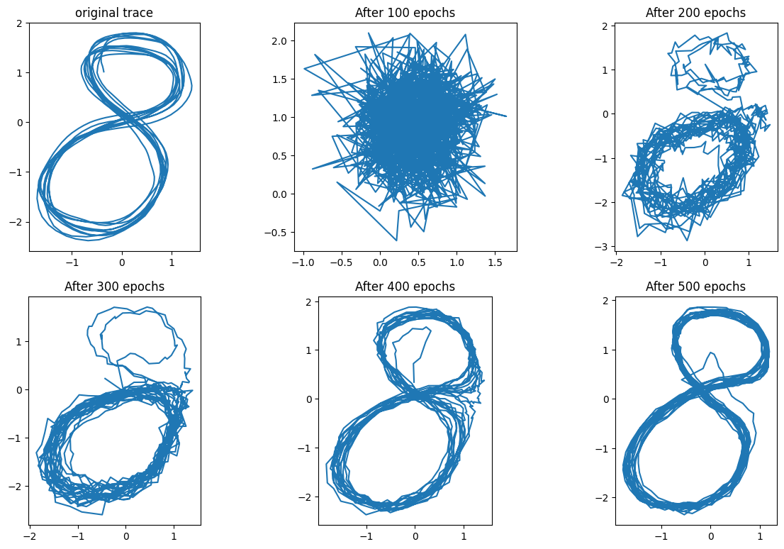
The success in generating this figure hid the fact that there was still a fundamental bug in my code. This bug came from the fact that a regular RNN cell predicts \(\mathbf{x}_{t+1} \approx \mathbf{\hat{x}}_t\) given \(\mathbf{x}_t\) at time $t$, so the reconstruction error is the sum of elements like \(\| \mathbf{\hat{x}}_t - \mathbf{x}_{t+1} \|^2\). On the other hand, the VRNN tries to reproduce \(\mathbf{x}_t \approx \mathbf{\hat{x}}_t\) at time step $t$ given \(\mathbf{h}_{t-1}\). The reconstruction error thus has terms like \(\|\mathbf{x}_t - \mathbf{\hat{x}}_t \|^2\). My mistake was to use errors like \(\| \mathbf{\hat{x}}_t - \mathbf{x}_{t+1} \|^2\). Since $\mathbf{x}_t$ and \(\mathbf{x}_{t+1}\) are usually close the model “kind of worked”, and recognizing that there was an error took me a while.

In the Appendix below I go through the sequence of experiments and ideas I had as the model failed to work well. When things went wrong I had to think about the VRNN and why it works, so the time wasn’t totally wasted. Also, this led me to set the adaptive $w$ ratio to $\frac{w \cdot DE}{RE} \approx 10$, which seems to produce good results.

A basic result

In this first experiment the VRNN does something new: it changes its precision depending on the context:

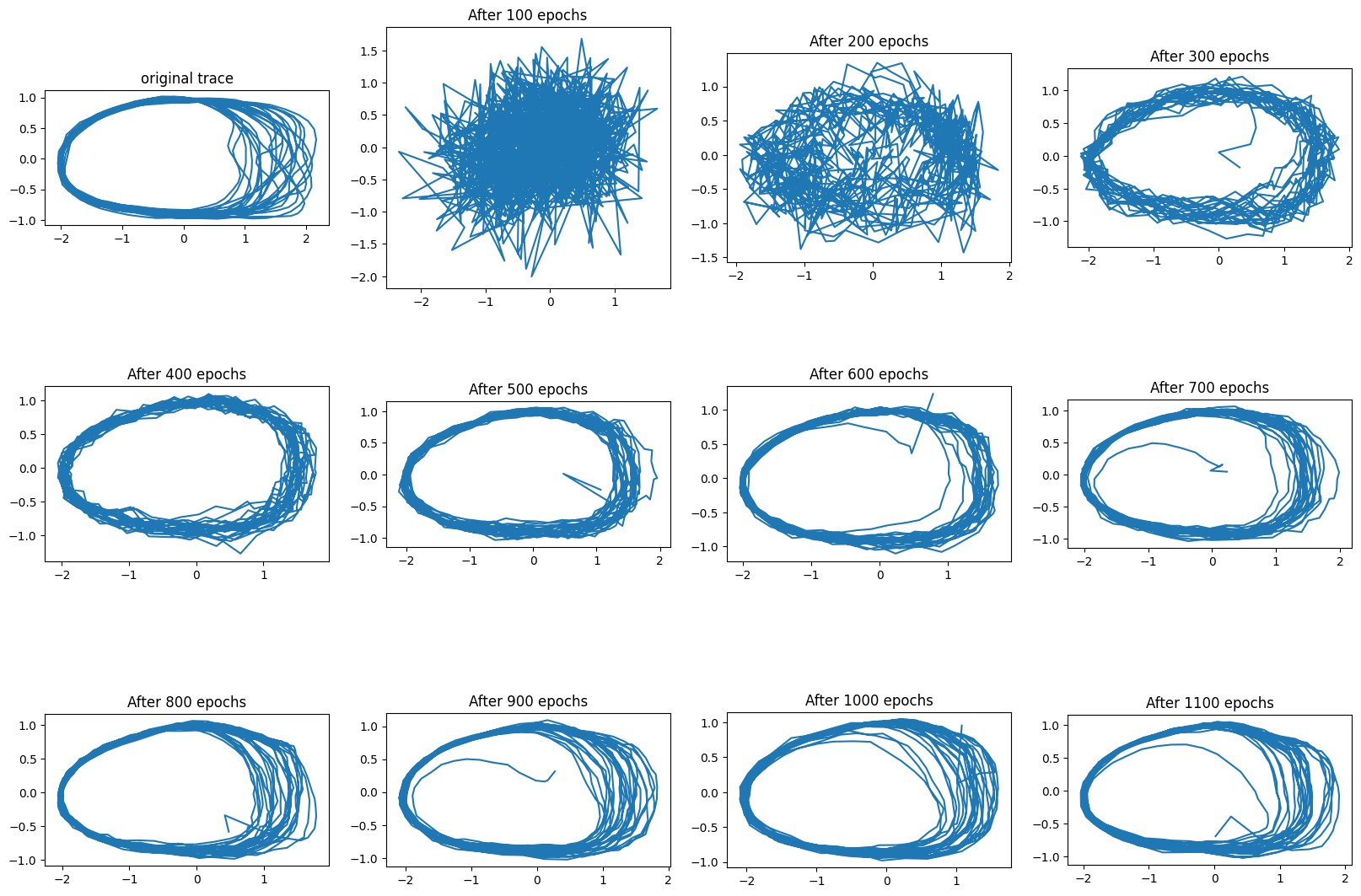
In the original trace that we are trying to reproduce, the left side of the oval has much less variance than the right side. To some extent this is captured by the traces generated with the VRNN after enough training.

Mixed results

The next experiment I tried reproducing a stochastic “eye” pattern, using GRU units.

In this pattern the wide oval is traced with probability 2/3, and the thin oval with probability 1/3, with transitions happening at the top, near the x=0, y=1 coordinate.

As can be seen, the VRNN does not seem to have two patterns which it switches stochastically. It seems to have a single pattern that approaches the original trace to some extent. Curiously, the reconstruction loss did get really low, which led me to wonder how well this network could reconstruct the original trace, mostly working as an autoencoder. If you reconstruct the trace using the “inference” mechanism (the one using during training) the reconstruction is quite close to the original.

So with the right context the network can produce the pattern, but the generation mechanism is at this point insufficient. Reminiscent of the issues I had with the VAE, the VRNN seemed to be ignoring the latent variable $\mathbf{z}$, and working like a regular RNN.

The VAE “optimization challenge” versus the VRNN optimization issues

In my VAE post I mentioned Bowman et. al 2015. In this paper it is pointed out that when training the VAE it is common that the $q(\mathbf{z} \vert \mathbf{x})$ parameters you learn tend to become equal to those of the $p(\mathbf{z})$ prior, so the KL divergence error is almost zero, and $\mathbf{z}$ does not get used. The VAE, however, is a different architecture from the VRNN. The VRNN is also different from architectures that use a VAE with a RNN in the encoder and/or the decoder (e.g. Bowman et. al 2015, or Chen et al. 2017). The question is: does the optimization challenge of VAEs surface somehow in VRNNs? Is this what I was facing?

In the case of the VAE optimization challenge, the posterior distribution of the latent variable “collapsed” into the prior due to the KL divergence term in the loss function. In the case of the VRNN the posterior and the prior are both functions of the hidden state \(\mathbf{h}_{t-1}\), and although the KL divergence term still encourages the prior \(\varphi_\tau^{prior}(h_{t-1})\) to resemble the posterior \(\varphi_\tau^{enc}(\varphi_\tau^{x}(\mathbf{x}_t), h_{t-1})\), in my simulations the error from the KL term was relatively large, whereas the reconstruction error was very small. The figure above (original trace vs inferred trace) shows this. The problem I had did not resemble the VAE optimization challenge in these regards.

The latent variable \(\mathbf{z}_t\) does seem to capture information about \(\mathbf{x}_t\), but it doesn’t seem to encode the “random structure” of the pattern, which in the above example could mean whether we are tracing a wide or a narrow circle. By using a relatively high-dimensional $\mathbf{z}$ value I was allowing the encoder to maintain all the information about $\mathbf{x}$, and by using a relatively large and powerful \(\varphi_\tau^{enc}\) network I was allowing it to simply invert whatever transformation the encoder was doing, driving the reconstruction error down.

A possible solution was therefore to reduce the dimension of $\mathbf{z}$, and use less powerful encoder and decoder networks.

Appendix: experiments with a “predictive” VRNN

As described above, my VRNN implementation calculated the reconstruction loss incorrectly. In code:

x, pmu, psig, mu, sig = vrnn(coords[:-1])
RE = mse_loss(x, coords[1:])

So the loss function used a shift in the input coordinates, as is common in autoregressive models. But this should not be done with the VRNN.

So I had just reproduced the figure 8 as shown previously. The interesting part was whether I would succeed with the “circle triangle eight” pattern.

Here is how it looked (1000 points are generated for each trajectory below):

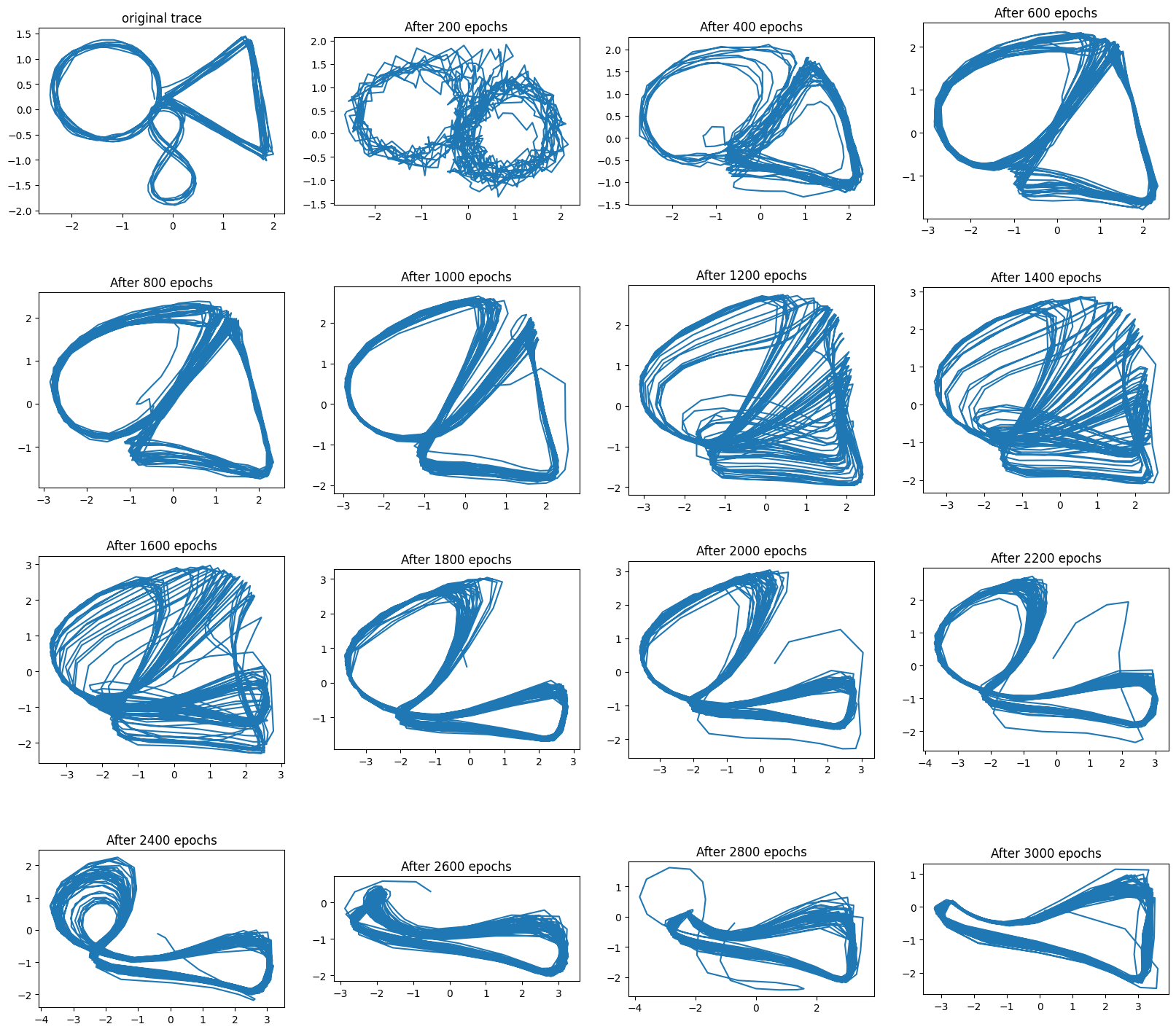
The impression I had is that the transition points between patterns are far and few, so it is hard for the network to learn proper $\mathbf{z}_t$ representations. Basically, it is easier to just learn a single trajectory that approaches the points of the single example I provided for the network to learn.

The first modification I used was to use GRU units for the $f_\theta$ network, which may help remember back to the transition points. I hoped that this and a large number of training epochs would do the trick. It did not, so I was left to wonder what was the problem.

I wanted the decoder to produce 3 attractors (circle, triangle, eight), and to switch between them based on the latent variable $\mathbf{z}_t$, which would potentially change its value when two cycles of the B pattern (the triangle) were completed. Instead I found a single attractor contorting its shape to match the original trace.

It didn’t seem like the latent variable was learning the transition points between patterns, and this should not be so surprising considering how sparse they are. My next move was to increase the training data, introducing 8 traces, each one with 5 to 10 transitions between patterns. This, together with GRU units, a VRNN with large layers, and enough training epochs should do the trick…

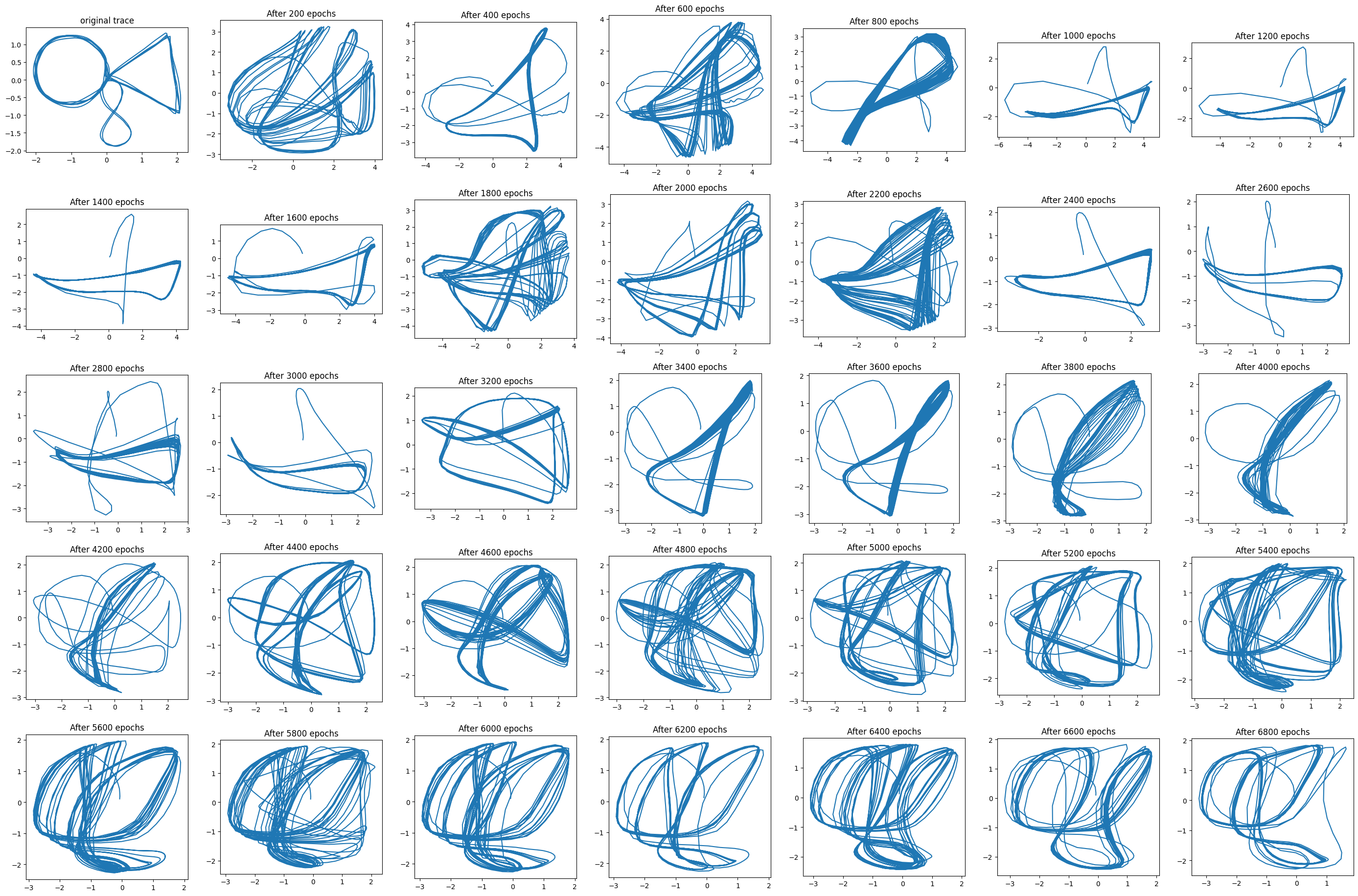
No, it didn’t do the trick. What now?

One thing I noticed is that the loss had become really small ($\approx$ 0.0001), both for the reconstruction error, and for $w$ times the KL divergence. The loss in the distribution of $\mathbf{z}$ was small, and yet the performance was poor. Perhaps setting $w$ so that $\frac{w \cdot DE}{RE} \approx 1$ was not so good in this case (see the VAE post). As a first variation I tried to set the initial $w=0$ value, and then adjust $w$ adaptive to approach the ratio $\frac{w \cdot DE}{RE} \approx 10$.

Another observation is that the circle-triangle-eight trajectory with two cycles of each shape is a challenging figure to trace. Given my lack of success, it may be better to try a simpler pattern, which I did.

For the next round of attempts I used the following “eye” pattern:

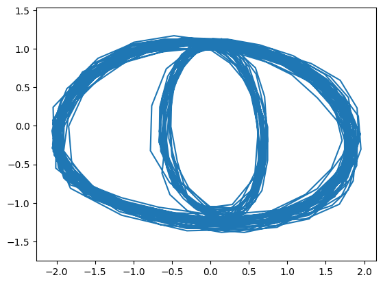
In this pattern when the pen is at the top, with probability 2/3 a wide oval will be traced, and with probability 1/3 a thin oval will be traced. Around 30 of these transitions were included in a single figure. Results from learning this pattern can be seen below.

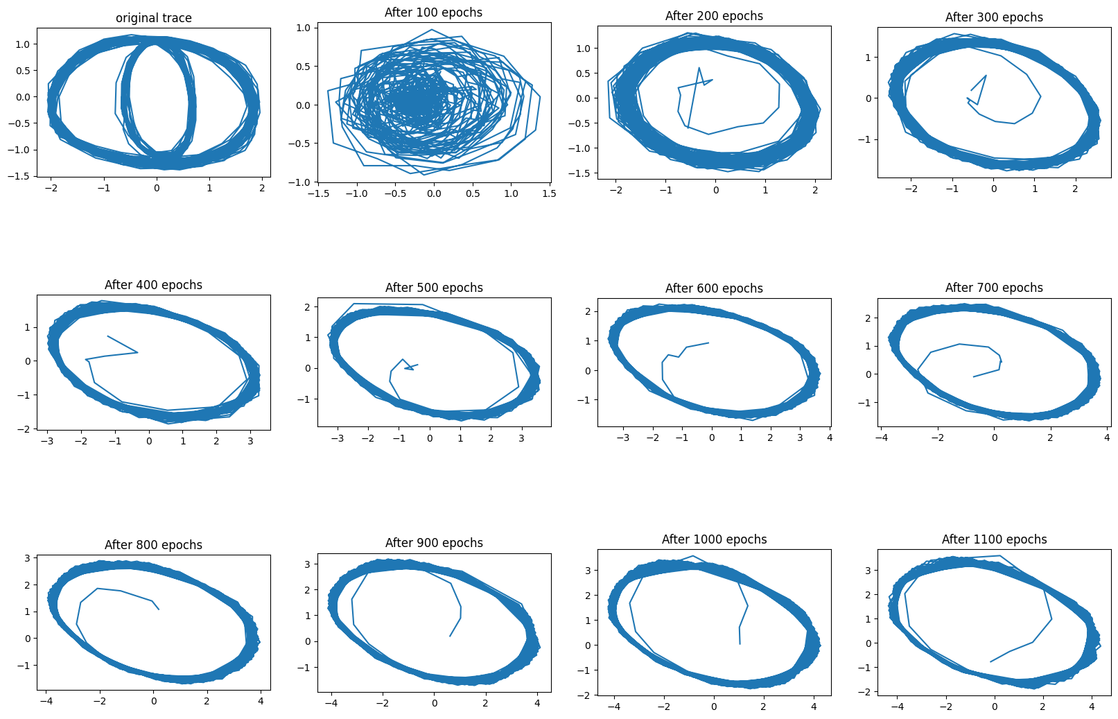
A this point I had this thought: a network that only traces the wide oval will reduce the loss just as much as a network that traces the wide oval with probability 2/3, and the thin oval with probability 1/3.

Because generation is stochastic, a “perfect” model only has probability 5/9 of matching the training data on any given cycle: the model matches the training data when 1) both are wide (with probability 4/9), and 2) both are thin (with probability 1/9). On the other hand, a “lazy” model that only traces the wide ovals will match the training data 66% of the time. This argument ignores differences in the phase caused by the thin oval being smaller, but those should be similar for both models.

In light of this, the reconstruction loss is not sufficient for learning the type of model we desire. Something must pressure the discovery of “transitions between patterns” at particular points. The question is why \(\text{KL}(q(\mathbf{z}_t \vert \mathbf{x}_{\leq T}, \mathbf{z}_{< T}) \|p(\mathbf{z}_t \vert \mathbf{x}_{< T}, \mathbf{z}_{< T}))\), should be able to do this. As far as I can tell, it can’t. You really need \(\mathbb{E}_{q(\mathbf{z}\leq T \vert \mathbf{x}\leq T)} \Big[ \text{KL}(q(\mathbf{z}_t \vert \mathbf{x}_{\leq T}, \mathbf{z}_{< T}) \|p(\mathbf{z}_t \vert \mathbf{x}_{< T}, \mathbf{z}_{< T})) \Big]\), or in other words, a long number of training epochs with small learning rates.